Contextualized Messages Boost Graph Representations

May 27 2024

Our paper Contextualized Messages Boost Graph Representations has recently been posted on arXiv (April 2025 update: published in TMLR). While the main theoretical results are presented in the paper, this post aims to provide an intuitive understanding of the motivation and findings. In summary, the paper theoretically justifies the need for anisotropic (i.e., a function of both the features of the center and neighboring nodes) and dynamic (i.e., a universal function approximator) message functions in graph neural networks (GNNs) and proposes a simple and computationally efficient model, the soft-isomorphic relational graph convolution network (SIR-GCN), satisfying this requirement that empirically outperforms comparable models.

1. Graph Neural Networks
   1. Graph Convolution Network (GCN)
   2. Graph Sample and Aggregate (GraphSAGE)
   3. Graph Attention Network (GAT)
   4. Graph Isomorphism Network (GIN)
   5. Principal Neighborhood Aggregation (PNA)
2. Soft-Isomorphic Relational Graph Convolution Network (SIR-GCN)
   1. Implementation
3. Experimental Results
4. Conclusion

Before delving into the paper and its main results, let us first review GNNs and how they operate.

Graph Neural Networks

Let $\mathcal{G} = \left(\mathcal{V}, \mathcal{E}\right)$ be a graph and $\mathcal{N}(u) \subseteq \mathcal{V}$ the set of nodes adjacent to node $u \in \mathcal{V}$. Suppose $\mathcal{H}$ is the space of node features and $\boldsymbol{h_u} \in \mathcal{H}$ is the feature of node $u$. A GNN following the message-passing scheme first aggregates the features of each node’s neighbors and then combines them to create an updated node feature. This can be expressed mathematically as $$\begin{aligned} \boldsymbol{H_u} &= \left\{\!\!\left\{\boldsymbol{h_v} : v \in \mathcal{N}(u)\right\}\!\!\right\} \\ \boldsymbol{a_u} &= AGG\left(\boldsymbol{H_u}\right) \\ \boldsymbol{h^*_u} &= COMB\left(\boldsymbol{h_u}, \boldsymbol{a_u}\right) \end{aligned}$$

where AGG and COMB are some aggregation and combination strategies, respectively, $\boldsymbol{H_u}$ is the multiset of neighborhood features for node $u$, $\boldsymbol{a_u}$ is the aggregated neighborhood feature for node $u$, and $\boldsymbol{h^*_u}$ is the updated feature for node $u$. An illustration is provided below.

Message-passing scheme for GNNs.

Since AGG takes arbitrary-sized multisets of neighborhood features as input and transforms them into a single feature, it may be considered a hash function. Hence, aggregation and hash functions shall be used interchangeably.

To provide additional context, five key GNNs in literature are introduced below.

Graph Convolution Network (GCN)

The graph convolution network (GCN) is one of the classical GNNs in literature. It can be expressed mathematically as $$\boldsymbol{h^*_u} = \sum_{v \in \mathcal{N}(u)} \dfrac{1}{\sqrt{\left|\mathcal{N}(u)\right|}\sqrt{\left|\mathcal{N}(v)\right|}} \boldsymbol{W} \boldsymbol{h_v}$$

where $\boldsymbol{W}$ represents a linear transformation of the neighborhood features $\boldsymbol{h_v}$.

Graph Sample and Aggregate (GraphSAGE)

The graph sample and aggregate (GraphSAGE) is another classic GNN designed for inductive representation learning. GraphSAGE with max pooling can be expressed as $$\boldsymbol{h^*_u} = \max_{v \in \mathcal{N}(u)} \left\{\sigma\left(\boldsymbol{W}\boldsymbol{h_v} + \boldsymbol{b}\right)\right\}$$

where $\boldsymbol{W}$ and $\boldsymbol{b}$ represents a linear transformation of the neighborhood features $\boldsymbol{h_v}$ and $\sigma$ is a non-linear activation function.

Graph Attention Network (GAT)

The graph attention network (GAT) leverages the popular attention mechanism to dynamically assign weights to each neighborhood feature. GATv2 can be expressed as $$\begin{aligned} \boldsymbol{h^*_u} &= \sum_{v \in \mathcal{N}(u)} \alpha_{u,v} \cdot \boldsymbol{W} \boldsymbol{h_v} \\ \alpha_{u,v} &= \dfrac{\exp\left(e_{u,v}\right)}{\sum_{w \in \mathcal{N}(u)} \exp\left(e_{u,w}\right)} \\ e_{u,v} &= \boldsymbol{a}^\top \text{LeakyReLU}\left(\boldsymbol{W_Q}\boldsymbol{h_u} + \boldsymbol{W_K}\boldsymbol{h_v}\right) \end{aligned}$$

where $\boldsymbol{W}$ represents a linear transformation of the neighborhood features $\boldsymbol{h_v}$ and $\boldsymbol{a}, \boldsymbol{W_Q}, \boldsymbol{W_K}$ jointly represents the attention mechanism.

Graph Isomorphism Network (GIN)

The graph isomorphism network (GIN) is designed to be a maximally powerful GNN when the space of node features is countable. It is based on the Weisfeiler Lehman (WL) graph isomorphism test. GIN can be expressed as $$\boldsymbol{h^*_u} = MLP\left((1 + \epsilon) \cdot \boldsymbol{h_u} + \sum_{v \in \mathcal{N}(u)} \boldsymbol{h_v}\right)$$

where $\epsilon$ is a scalar that may be learnable and MLP is a multi-layer perceptron.

For more details about countable and uncountable sets, see Wikipedia.

Principal Neighborhood Aggregation (PNA)

The principal neighborhood aggregation (PNA) is a recently proposed GNN designed to be maximally expressive when the space of node features is uncountable. It can be expressed as $$\boldsymbol{h^*_u} = \bigoplus_{v \in \mathcal{N}(u)} \left[\boldsymbol{W_Q} \boldsymbol{h_u} + \boldsymbol{W_K} \boldsymbol{h_v}\right]$$

where $\bigoplus$ comprises multiple aggregators (e.g., mean, standard deviation, max, and min) and $\boldsymbol{W_Q}, \boldsymbol{W_K}$ are linear transformations of the center node features $\boldsymbol{h_u}$ and neighborhood features $\boldsymbol{h_v}$, respectively.

Technically speaking, PNA also introduces scalars as part of the aggregators $\bigoplus$. We ignore this for ease of discussion.

Soft-Isomorphic Relational Graph Convolution Network (SIR-GCN)

Based on the models introduced above, we can formulate the hash function in the message-passing framework as $$G\left(\boldsymbol{H}\right) = \sum_{\boldsymbol{h} \in \boldsymbol{H}} g\left(\boldsymbol{h}\right)$$

where $g$ is the feature map or message function transforming the features of neighboring nodes $\boldsymbol{h} \in \boldsymbol{H}$. Notably, the majority of existing GNNs simply use a linear message function $g$, resulting in a linear hash function with respect to the neighborhood features.

Intuitively, the sum aggregation may also be replaced with the mean, symmetric mean, or max aggregation.

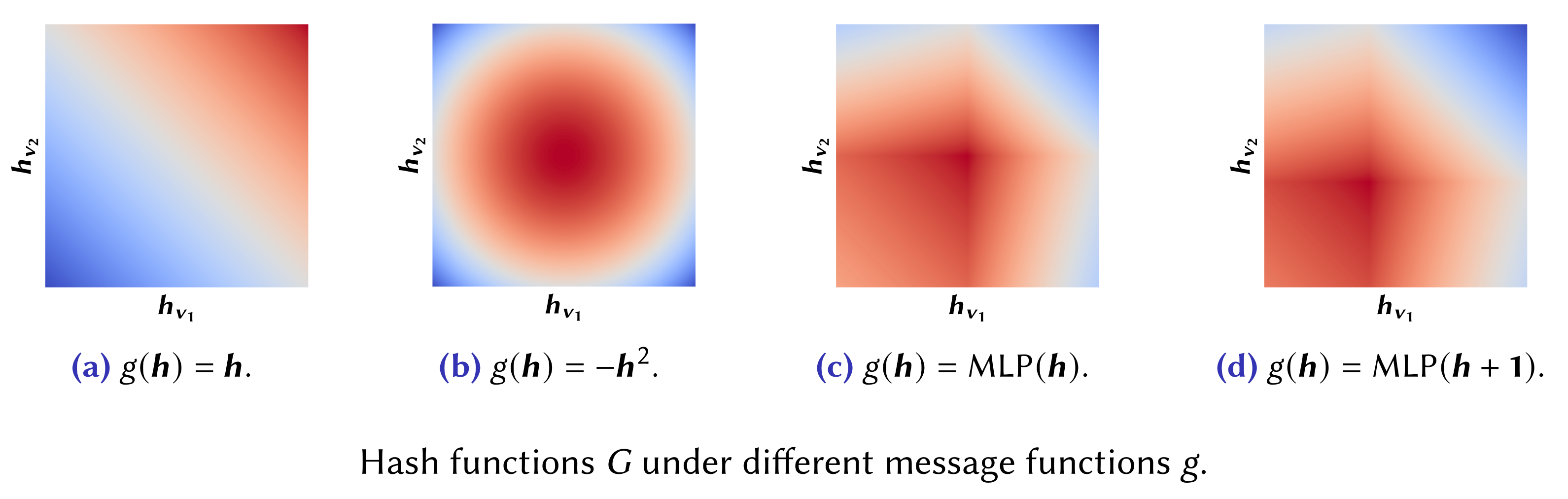
To illustrate the limitations of existing models, consider node $u$ with two neighbors $v_1$ and $v_2$ and the task of anomaly detection on the scalar node features $\boldsymbol{h_{v_1}}$ and $\boldsymbol{h_{v_2}}$ representing zero-mean scores. If $g$ is linear, the corresponding contour plot of the hash function $G$ in Figure (a) below highlights collisions—instances where distinct inputs produce identical outputs—between dissimilar multisets of neighborhood features, resulting in aggregated neighborhood features that are less useful for the task. For instance, both $\boldsymbol{H_{u}^{(1)}} = \left\{0, 0\right\}$ and $\boldsymbol{H_{u}^{(2)}} = \left\{-10, 10\right\}$ will produce an aggregated neighborhood feature of $\boldsymbol{a_{u}} = 0 + 0 = -10 + 10 = 0$ even if they are intuitively dissimilar.

Hash collisions in GNNs.

In contrast, for more complex message functions $g$, the corresponding hash function $G$ becomes non-trivial and possibly more meaningful. For instance, if $g\left(\boldsymbol{h}\right) = - \boldsymbol{h}^2$, then the corresponding hash function $G$ in Figure (b) produces hash collisions that are more useful and intuitive for detecting anomalous scores. In practice, this may be achieved by applying activation functions or MLPs before or after each GNN layer to induce non-linearity in $g$.

Nevertheless, this approach still has its limitations. Specifically, since the message function $g$ is solely a function of the neighborhood features $\boldsymbol{h_v} \in \boldsymbol{H_u}$, the complex relationship between neighboring nodes cannot be learned. Figures (c) and (d) provide intuition for the necessity of $g$ to consider both the features of the center and neighboring nodes: for nodes $u \neq u' \in \mathcal{V}$ having the same two neighbors $v_1$ and $v_2$ with $\boldsymbol{h_u} \neq \boldsymbol{h_{u'}}$, the introduction of the bias term $\boldsymbol{0}$ and $\boldsymbol{1}$ (assuming a function of the center node features $\boldsymbol{h_u}$ and $\boldsymbol{h_{u'}}$) results in distinct aggregated neighborhood features $\boldsymbol{a_u} \neq \boldsymbol{a_{u'}}$ even if the multiset of neighborhood features are identical $\boldsymbol{H_u} = \boldsymbol{H_{u'}}$. This approach makes the message function $g$ and hash function $G$ adaptive with respect to the features of the center node $u$, allowing it to learn the relationship between nodes connected by an edge to produce contextualized aggregated neighborhood features.

In the event that $\boldsymbol{h_u} = \boldsymbol{h_{u'}}$ for nodes $u \neq u'$, one may inject stochasticity into the node features to distinguish between nodes with identical features and neighborhood features with high probability (Sato et al.).

In line with this observation, we emphasize the need for a dynamic (i.e., a universal function approximator) message function that takes both the features of the center and neighboring nodes as input (i.e., anisotropic). By the universal approximation theorem, this message function $g$ may be modeled as a two-layer MLP resulting in the soft-isomorphic relational graph convolution network (SIR-GCN) $$\boldsymbol{h_u^*} = \sum_{v \in \mathcal{N}(u)} \boldsymbol{W_R} ~ \sigma\left(\boldsymbol{W_Q} \boldsymbol{h_u} + \boldsymbol{W_K} \boldsymbol{h_v}\right)$$

where $\sigma$ is a non-linear activation function, $\boldsymbol{W_Q}, \boldsymbol{W_K} \in \mathbb{R}^{d_{\text{hidden}} \times d_{\text{in}}}$, and $\boldsymbol{W_R} \in \mathbb{R}^{d_{\text{out}} \times d_{\text{hidden}}}$. These jointly represent a contextualized (i.e., anisotropic and dynamic) message function. Leveraging linearity, the proposed model has a computational complexity of $$\mathcal{O}\left(\left|\mathcal{V}\right| \times d_{\text{hidden}} \times d_{\text{in}} + \left|\mathcal{E}\right| \times d_{\text{hidden}} + \left|\mathcal{V}\right| \times d_{\text{out}} \times d_{\text{hidden}}\right)$$

with computational efficiency achieved by the application of only an activation function along edges.

Our proposed model is analogous to the recently proposed Kolmogorov-Arnold Networks (KANs). Similar to KANs, instead of applying activation functions on nodes, SIR-GCN applies non-linearities along edges. This allows the model to “reason along an edge.”

Our paper also presents a mathematical discussion on the relationship between SIR-GCN and the key GNNs introduced above, establishing the former as a generalization of classical GNN methodologies. This highlights the novelty of SIR-GCN as the first GNN model to incorporate both anisotropic and dynamic messages. The discussion further demonstrates that SIR-GCN is comparable to a modified WL test in terms of graph isomorphism representational capability, thereby inheriting the theoretical properties of the WL test.

Implementation

The code for SIR-GCN using the Deep Graph Library (DGL) framework is provided below.

import torch
from torch import nn
from dgl import function as fn
from dgl.utils import expand_as_pair

class SIRConv(nn.Module):
    r"""Soft-Isomorphic Relational Graph Convolution Network (SIR-GCN)
    
    .. math::
        h_u^* = \sum_{v \in \mathcal{N}(u)} W_R \sigma(W_Q h_u + W_K h_v)

    Parameters
    ----------
    input_dim : int
        Input feature dimension
    hidden_dim : int
        Hidden feature dimension
    output_dim : int
        Output feature dimension
    activation : a callable layer
        Activation function, the :math:`\sigma` in the formula
    dropout : float, optional
        Dropout rate for inner linear transformations, defaults to 0
    inner_bias : bool, optional
        Whether to learn an additive bias for inner linear transformations, defaults to True
    outer_bias : bool, optional
        Whether to learn an additive bias for outer linear transformations, defaults to False
    agg_type : str, optional
        Aggregator type to use (``sum``, ``max``, ``mean``, or ``sym``), defaults to ``sum``
    """
    def __init__(self, input_dim, hidden_dim, output_dim, activation, dropout=0, inner_bias=True, outer_bias=False, agg_type='sum'):
        super(SIRConv, self).__init__()
        self.activation = activation
        self.dropout = nn.Dropout(dropout)
        self.linear_query = nn.Linear(input_dim, hidden_dim, bias=inner_bias)
        self.linear_key = nn.Linear(input_dim, hidden_dim, bias=False)
        self.linear_relation = nn.Linear(hidden_dim, output_dim, bias=outer_bias)

        self._agg_type = agg_type
        self._agg_func = fn.sum if agg_type == 'sym' else getattr(fn, agg_type)
    
    def message_func(self, edges):
        if self._agg_type in ['sum', 'mean', 'sym']:
            return {'m': edges.src['norm'] * edges.dst['norm'] * self.activation(edges.dst['eq'] + edges.src['ek'])}
        else: # Cannot leverage linearity for max aggregation
            return {'m': self.linear_relation(self.activation(edges.dst['eq'] + edges.src['ek']))}
        
    def forward(self, graph, feat):
        with graph.local_scope():
            degs = graph.in_degrees().float().clamp(min=1).to(graph.device)
            norm = torch.pow(degs, -0.5) if self._agg_type == 'sym' else torch.ones(graph.num_nodes(), device=graph.device)
            norm = norm.reshape((graph.num_nodes(),) + (1,) * (feat.dim() - 1))
            graph.ndata['norm'] = norm
 
            feat_key, feat_query = expand_as_pair(feat, graph)
            graph.ndata['ek'] = self.dropout(self.linear_key(feat_key))
            graph.ndata['eq'] = self.dropout(self.linear_query(feat_query))

            graph.update_all(self.message_func, self._agg_func('m', 'ft'))
            rst = graph.ndata.pop('ft')
            rst = self.linear_relation(rst) if self._agg_type in ['sum', 'mean', 'sym'] else rst
            
            return rst

SIR-GCN implementation in DGL.

Experimental Results

To highlight the contribution, we evaluated SIR-GCN on a subset of the Benchmarking GNNs, a collection of benchmark datasets consisting of diverse mathematical and real-world graphs across various GNN tasks. In particular, the WikiCS, PATTERN, and CLUSTER datasets fall under node property prediction tasks while the MNIST, CIFAR10, and ZINC datasets fall under graph property prediction tasks. Furthermore, the WikiCS, MNIST, and CIFAR10 datasets have uncountable node features while the remaining datasets have countable node features. The performance metric of ZINC is the mean absolute error (MAE) while the performance metric of the remaining datasets is accuracy. See Dwivedi et al. (2023) for more information regarding the individual datasets.

Model	WikiCS (↑)	PATTERN (↑)	CLUSTER (↑)	MNIST (↑)	CIFAR10 (↑)	ZINC (↓)
MLP	59.45 ± 2.33	50.52 ± 0.00	20.97 ± 0.00	95.34 ± 0.14	56.34 ± 0.18	0.706 ± 0.006
GCN	77.47 ± 0.85	85.50 ± 0.05	47.83 ± 1.51	90.12 ± 0.15	54.14 ± 0.39	0.416 ± 0.006
GraphSAGE	74.77 ± 0.95	50.52 ± 0.00	50.45 ± 0.15	97.31 ± 0.10	65.77 ± 0.31	0.468 ± 0.003
GAT	76.91 ± 0.82	75.82 ± 1.82	57.73 ± 0.32	95.54 ± 0.21	64.22 ± 0.46	0.475 ± 0.007
GIN	75.86 ± 0.58	85.59 ± 0.01	58.38 ± 0.24	96.49 ± 0.25	55.26 ± 1.53	0.387 ± 0.015
PNA	-	-	-	97.19 ± 0.08	70.21 ± 0.15	0.320 ± 0.032
SIR-GCN	78.06 ± 0.66	85.75 ± 0.03	63.35 ± 0.19	97.90 ± 0.08	71.98 ± 0.40	0.278 ± 0.024

Test performance on Benchmarking GNNs.

The table above presents the mean and standard deviation of the test performance for SIR-GCN and comparable GNNs across the six benchmarks where the experimental set-up follows that of Dwivedi et al. to ensure a fair evaluation. The results show that SIR-GCN consistently outperforms key GNNs in literature. Notably, SIR-GCN also outperforms PNA which uses multiple aggregators. This supports the intuition of utilizing anisotropic and dynamic messages to enhance the expressivity of GNNs.

Conclusion

Overall, we proposed a novel perspective for creating a powerful GNN when the space of node features is uncountable. Our theoretical results suggest the need for contextualized message functions, which allow the model to learn the relationship between the features of the center and neighbor nodes.

Let me know your thoughts!